Nsound FFT¶

Nsound currently implements its own fast Fourier transform (FFT) in C++. In the furture this will change and use the FFTW library if available.

The FFT is provided by the FFTransform class. It takes an input signal Buffer and transforms it into the frequency domain. The basic documentation:

FFTransform(sample_rate)¶

sample_rate: The number of samples per second. The sample rate is used for creating plots with correct axes.

FFTransform.fft(x, n_order)¶

x: The input Buffer.
n_order: The size of the FFT to perform.

Returns an FFTChunkVector, representing the input signal chopped up into frames, where each frame is n_order is size.

FFTransform.ifft(fft_chunk_vector)¶

fft_chunk_vector: The input FFTChunkVector returned by fft().

Returns an Buffer, where each FFTChunk in the FFTChunkVector is transformed back into the time-domain.

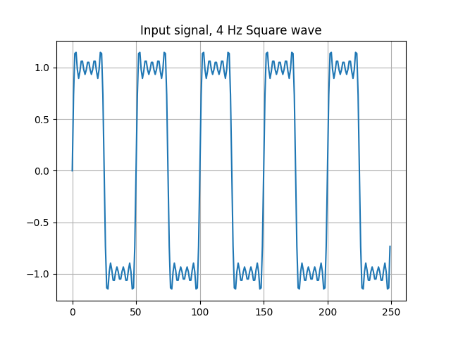
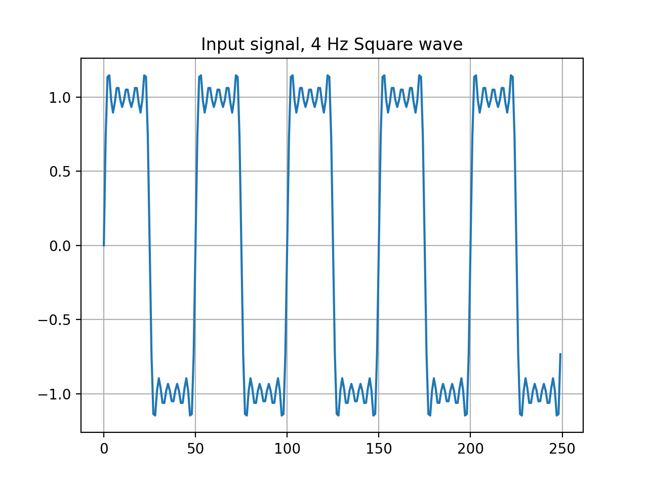
The example below creates a square wave with 5 harmonics.

import Nsound as ns

sample_rate = 500.0

square = ns.Square(sample_rate, 5)

b = ns.Buffer()
b << square.generate(0.5, 10.0)

fft = ns.FFTransform(sample_rate)

vec = fft.fft(b, 256)

b.plot("Input signal, 4 Hz Square wave")

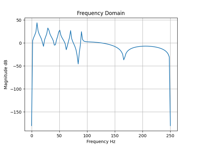
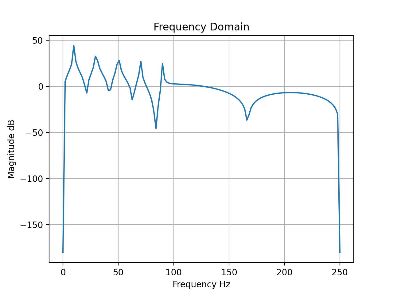
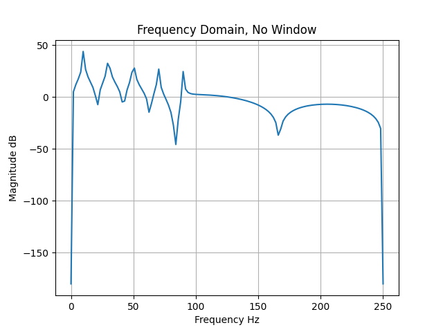
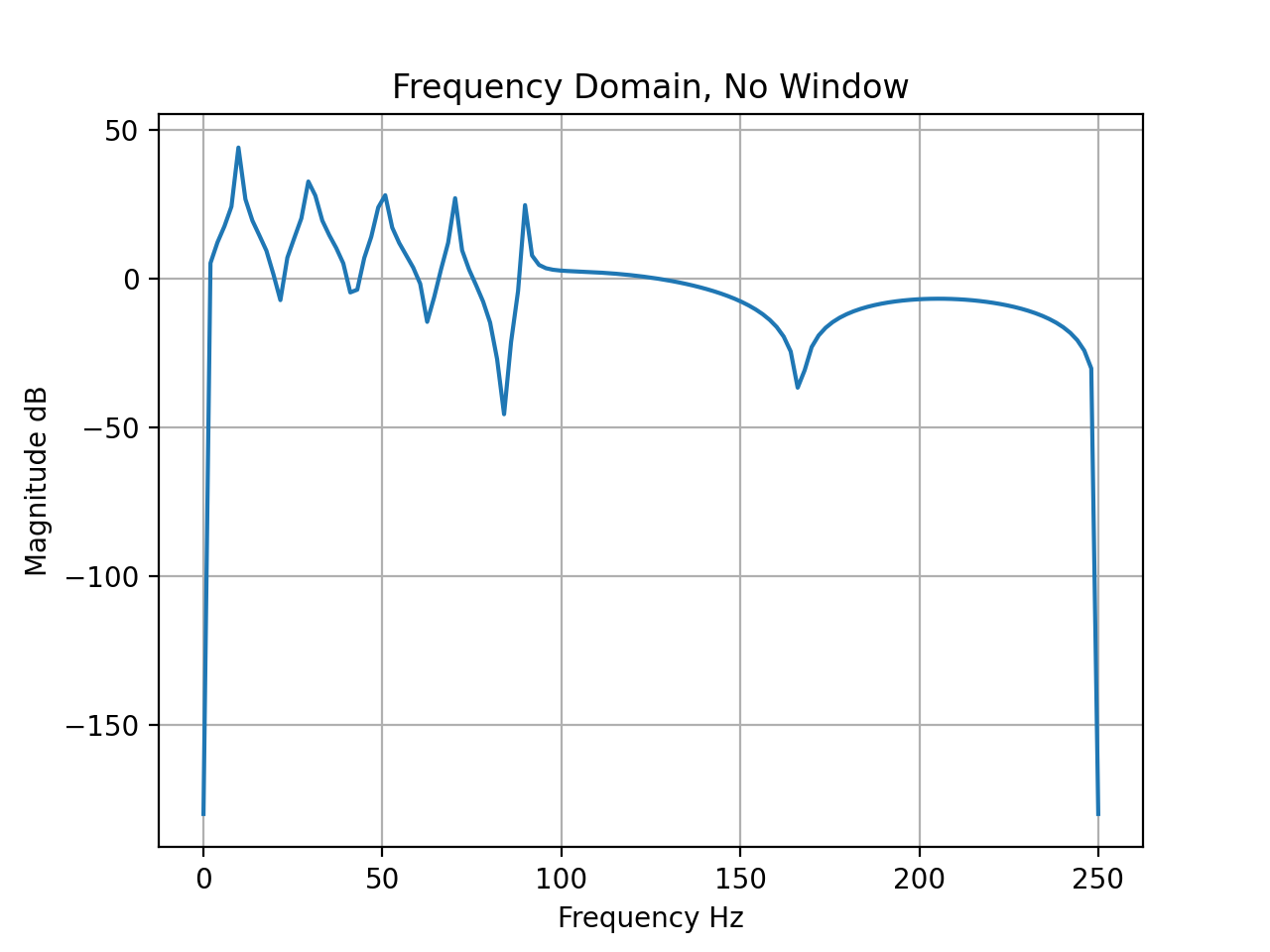
vec[0].plot("Frequency Domain")

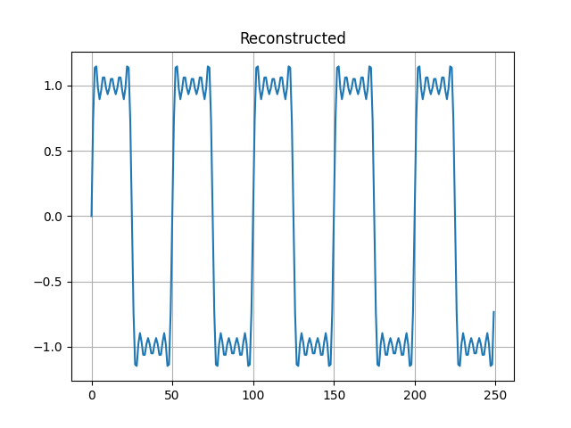
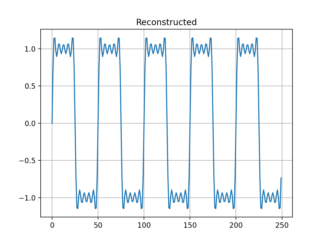
b2 = fft.ifft(vec)
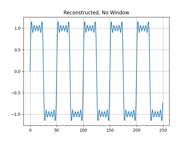
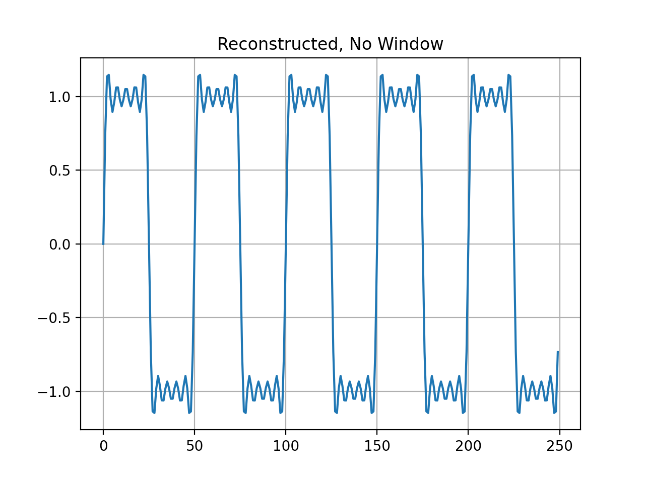
b2.plot("Reconstructed")

(Source code)

_images/fft-1_00.png — (png, hires.png, pdf)¶

_images/fft-1_01.png — (png, hires.png, pdf)¶

_images/fft-1_02.png — (png, hires.png, pdf)¶

Notice that there are 5 peaks, these correspond to the 5 harmonics in the square wave.

Using a Window¶

Setting a window on the FFT object can get rid of edge effects. This can improve the results when looking at the frequency domain, but it will affect the reconstructed signal.

import Nsound as ns

sample_rate = 500.0

square = ns.Square(sample_rate, 5)

b = ns.Buffer()
b << square.generate(0.5, 10.0)

fft = ns.FFTransform(sample_rate)

vec1 = fft.fft(b, 256)
b1   = fft.ifft(vec1)

fft.setWindow(ns.HANNING)

vec2 = fft.fft(b, 256)
b2   = fft.ifft(vec2)

vec1[0].plot("Frequency Domain, No Window")
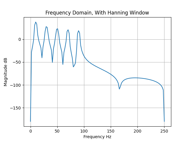
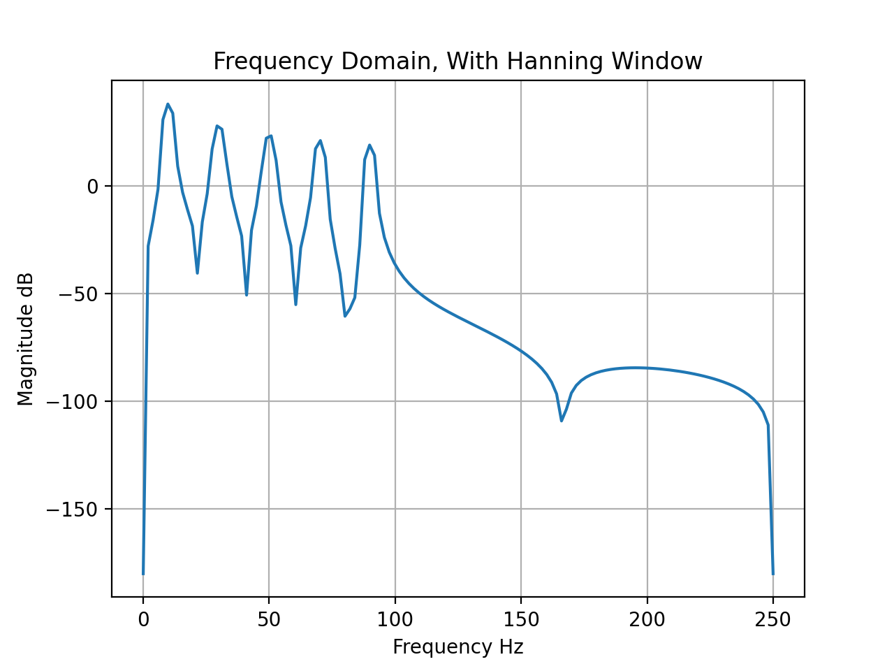
vec2[0].plot("Frequency Domain, With Hanning Window")

b1.plot("Reconstructed, No Window")
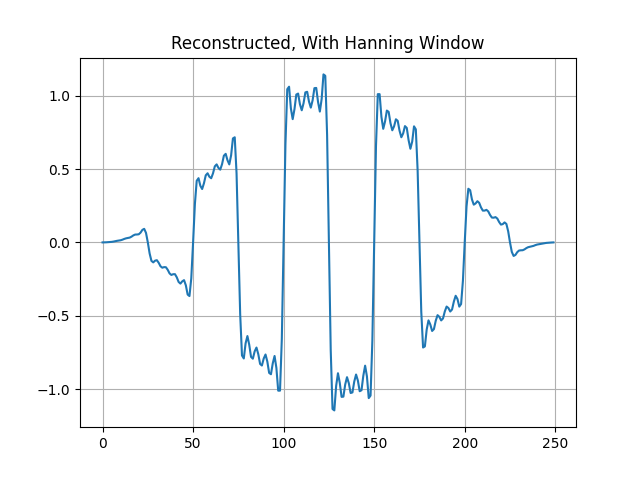
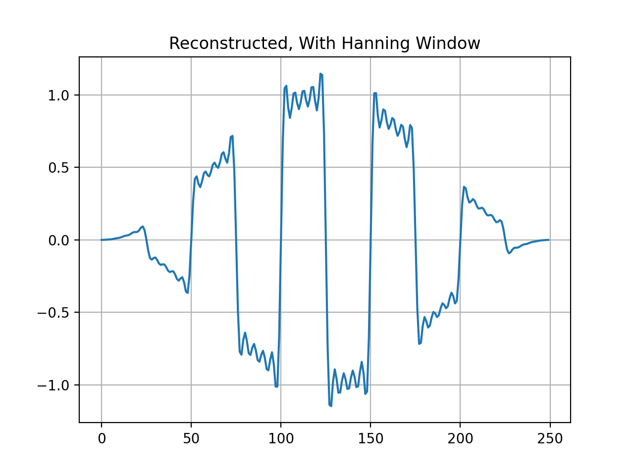
b2.plot("Reconstructed, With Hanning Window")