Gravity Wave Signal Processing
With all the excitement about LIGO and gravity waves, I’ve downloaded the raw GW150914 detection data for from here. The file I downloaded was 32 seconds sampled at 4096 samples per second.
Next I reviewed some of the LIGO tutorial on signal processing here, and proceeded to write a Python script using Nsound to process the data. Talk about finding a needle in a haystack!
Raw time-series data plot, the detection event occurs around 16.5 seconds in this plot:
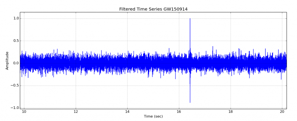
Where’s the signal? It’s buried in noise! Mostly low frequencies. But with the help of a band pass filter from 80 to 280 Hz, we can get a hint of the signal:
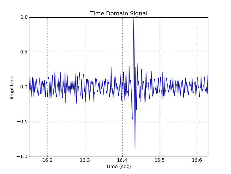
Zooming in:
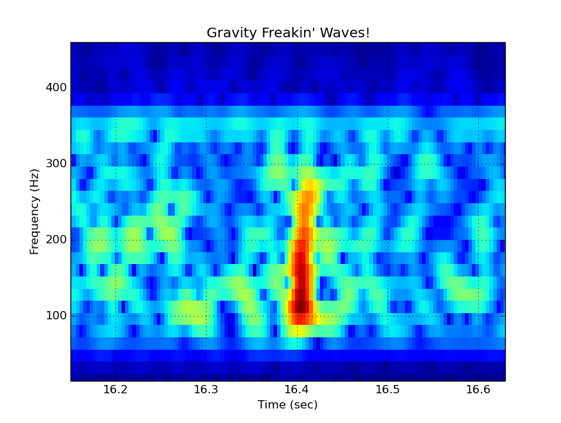
Plotting the spectrogram:
Audio
And finally, we can listen to the universe! The detection is a single blip as show above, however for your listening pleasure I’ve repeated the blip 4 times:
Link to the .wav here.
Python Code
Here is the Python code I used which uses my Nsound Python library:
|
1 2 3 4 5 6 7 8 9 10 11 12 13 14 15 16 17 18 19 20 21 22 23 24 25 26 27 28 29 30 31 32 33 34 35 36 37 38 39 40 41 42 43 44 45 46 47 48 49 50 51 52 53 54 55 56 57 58 59 60 61 62 63 64 65 66 67 68 69 70 71 72 73 74 75 76 77 78 79 80 81 82 83 84 85 86 87 88 89 90 91 92 93 94 95 96 97 98 99 |
""" Reads in the LIGO gravity wave data for GW150914, a file named 'H-H1_LOSC_4_V1-1126259446-32.txt', and performs a band pass filter from 80 to 280 Hz. The data are then written out to a .wav file so it can be played on a computer. By Nick Hilton 2016-02-11 """ import Nsound as ns plt = ns.Plotter() #------------------------------------------------------------------------------ # read in time series data with open('H-H1_LOSC_4_V1-1126259446-32.txt', 'r') as fd: lines = fd.readlines() sr = 4096.0 a = ns.AudioStream(sr, 1) for l in lines: l = l.strip() # skip comments if l.startswith('#'): continue s = float(l) a << s a.normalize() # The data don't start and end at zero so there's an initial step function, which # causes a big spike in the spectrogram. So I'm going to apply a Gaussian # window to smooth the start and stop of the data. dur = a.getDuration() gen = ns.Generator(sr) gau = gen.drawFatGaussian(dur, 0.99) while len(gau) < len(a): gau << 0.0 a *= gau #----------------------------------------------------------------------------- # band pass filter to region of interest bpf = ns.FilterBandPassIIR(sr, 5, 80, 280, 0.01) a2 = bpf.filter(a) a2.normalize() a2.plot('Filtered Time Series GW150914') plt.show() #----------------------------------------------------------------------------- # spectrogram spec = ns.Spectrogram(a2[0], sr, 0.0625, 0.0039, ns.PARZEN) spec.plot('Gravity Freakin\' Waves!', False, 0.5) # zoom in on region plt.xlim(16.15, 16.63) plt.ylim(15, 460) a2.plot('Time Domain Signal') # zoom in on region plt.xlim(16.15, 16.63) #------------------------------------------------------------------------------ # pull out 2 second around the gravity wave and repeat it several times for # playback a3 = a2.substream(16.0, 2.0) # remove any step function around the edges gau = gen.drawFatGaussian(2.0, 0.99) while len(gau) < len(a3): gau << 0.0 a3 *= gau a3 << a3 << a3 a3 >> "out.wav" ns.Plotter.show() |


